Neural Nets Understanding Language: Word2vec
Full notebook: https://www.kaggle.com/code/tonylu25/word2vec
I was in awe when I learned that we could represent words and sentences as mathematical representations.
But how does a vector encode semantics?
How is it possible that, mathematically, we can show: King - Man + Woman = Queen
When I implemented a RAG system for learning a book (https://github.com/tlulu/human_condition), I chunked up parts of the book, created embeddings for each chunk and stored them in a vector database.
Then the query gets transformed into an embedding.
Only similar chunks related to the query embedding are returned.
But that’s sentence/paragraph embeddings.
I even didn’t understand how a single word embedding worked..
Here I implemented Word2Vec, after understanding the concepts from this amazing blog by Chris McCornick.
Let’s use the definition of “social media “from https://www.apa.org/topics/social-media-internet as our corpus.
corpus = """
Social media are forms of digital communication through
which users create online communities to share information,
ideas, personal messages, and other content.
Social media use is not inherently beneficial or harmful.
Social media platforms offer powerful opportunities for socialization and connection,
but may also have some negative effects, including mis- and disinformation,
hate speech, and cyberbullying. At the extreme, social media use can interfere with sleep,
physical activity, and in-person social interactions.
"""
The idea is simple: Words that are nearby each other in proximity will have a stronger relationship than words that aren’t.
Like “social” and “interaction” will be more closely related than “dog” and “motor”.
It turns out (spoiler alert),
the embeddings are the weights after training our neural net.
The input to the neural net are pairs of words that have close proximity to each other.
Proximity is a strong indicator that words are related.
The model’s output is the list of probabilities of the next word.
We first tokenize the corpus, isolating each word, stripping away punctuation and extra white spaces
def tokenize(corpus):
    return re.findall(r"\w+(?:'\w+)?", corpus.lower())
Then we create our vocabulary list, of distinct words, with an index to track each word. Our neural net returns this list along with their respective probabilities as the next word.
vocabulary = list(set(tokens))

def build_mapping(vocabulary):
    map = {}
    for i in range(len(vocabulary)):
        map[vocabulary[i]] = i
    return map

word_mapping = build_mapping(vocabulary) # words to indices in vocabulary list
Next we build our training data.
We build a list of tuples for every word and its neighbors.
window_size = 2
def build_training_data(tokens):
    training_data = []
    for i in range(len(tokens)):
        current = tokens[i]
        for j in range(window_size):
            if i + j + 1 < len(tokens):
               training_data.append((current, tokens[i + j + 1]))
            if i - j - 1 >= 0:
               training_data.append((current, tokens[i - j - 1]))

    return training_data

training_data = build_training_data(tokens)

=>

[('social', 'media'),
 ('social', 'are'),
 ('media', 'are'),
 ('media', 'social'),
 ('media', 'forms'),
 ('are', 'forms'),
 ('are', 'media'),
 ...
I transform the training data into labels for our neural net.
The inputs and target outputs are one hot encodings using our vocabulary list.
X = []
y = []
for j in range(len(training_data)):
    x_index = word_mapping[training_data[j][0]]
    x_onehot = torch.zeros(len(vocabulary))
    x_onehot[x_index] = 1.0
    X.append(x_onehot)

    target_index = word_mapping[training_data[j][1]]
    target_onehot = torch.zeros(len(vocabulary))
    target_onehot[target_index] = 1.0
    y.append(target_onehot)

X = torch.stack(X)
y = torch.stack(y)

print(f"{len(X)} {len(X[0])}")
print(f"{len(y)} {len(y[0])}")

=>

286 61
286 61
Great - there are 286 pairs of training data, each one hot encoding is of length 61, which is the size of our vocabulary.
For our neural net, we initialize a hidden layer with 10 neurons.
Google used 300 features in their published model trained on the Google news dataset.
But for our tiny corpus, 10 is enough. In fact, the training breaks down with 300 neurons.
input_layer_size = len(vocabulary)
output_layer_size = input_layer_size
hidden_layer_neurons = 10

class NeuralNet(nn.Module):
    def __init__(self):
        super().__init__()
        self.layer1 = nn.Linear(input_layer_size, hidden_layer_neurons)
        self.layer2 = nn.Linear(hidden_layer_neurons, output_layer_size)

        nn.init.normal_(self.layer1.weight.data, mean=0.0, std=1.0)
        nn.init.normal_(self.layer2.weight.data, mean=0.0, std=1.0)

    def forward(self, x):
        x = self.layer1(x)
        x = self.layer2(x)
        x = torch.softmax(x, dim=1)
        return x

# p is the actual probability and q is the probability output from our model.
def cross_entropy_loss(p, q):
   return -(p * torch.log(q)).sum(dim=1).mean()

model = NeuralNet()

train_loss = []
iterations = 30000
learning_rate = 0.05
for i in range(iterations):
    output = model(X)

    model.zero_grad()
    loss = cross_entropy_loss(y, output)
    loss.backward()
    train_loss.append(loss.item())

    with torch.no_grad(): # Tell pytorch to not do any gradient updating in the background.
        for p in model.parameters():
            p -= learning_rate * p.grad
Plotting the loss over time, we see that training has been successful.
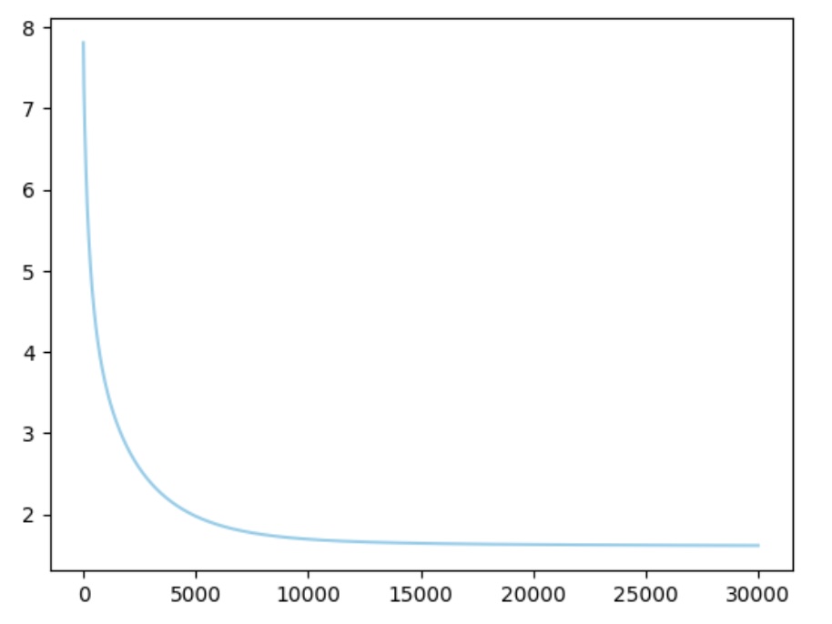
The structure for back-propgation is similar to the neural net for recognizing digits.
However, there are some interesting details here.
Initializing weights
By default, pytorch initializes weights within [-0.1, 0.1].
We’d get this graph if we didn’t initialize the weights with greater values nn.init.normal_(self.layer1.weight.data, mean=0.0, std=1.0)
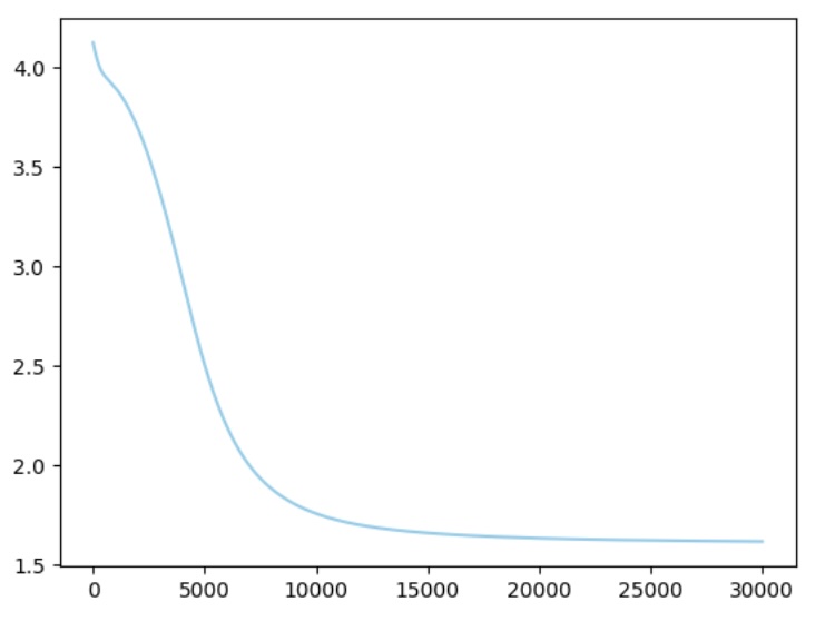
My interpretation is that because the weights are smaller, the gradient is smaller, making the drop is a lot less sharp.
Loss function
For the loss function, we use cross entropy loss, a way of measuring how surprised our model is when predicting reality.
P is the probability distribution from our labeled data (reality)
Q is the probability distribution of the outputs from our model.
This sounded really abstract at first.
Let’s break down this formula to get a better intuition.
This formula indicates surprise.
The more unlikely an event is, the higher the surprise.
Entropy is defined as the weighted average of surprise across the distribution
For each event, cross entropy is the surprise from our model multiplied by how often it appears in reality.
For example, if we had a fair coin (0.5 tails, 0.5 heads) in reality but our model predicted that of a broken coin (0.1 tails, 0.9 heads), we’d have a cross entropy of 0.5 * ln(1/0.1) + 0.5 * ln(1/0.9) = 1.2 for one flip.
But if our model modeled a fair coin, the cross entropy would be 0.5 * ln(1/0.5) + 0.5 * ln(1/0.5) = 0.69 which is the ideal number.
So in training, we’re essentially trying to make the model's distribution match reality's distribution by bringing down the entropy.
With Word2vec, the model is initialized with random weights.
The reality distribution comes from our labeled training data.
With this, we have created a mathematical representation for a word!
embeddings = model.layer1.weight.data

def get_embedding(word):
    idx = word_mapping[word]
    return model.layer1.weight[:, idx].data

print(get_embedding("social"))

=>
tensor([-0.8526,  0.8450, -2.3760, -2.5202, -0.2360,  1.4085, -0.9876,  1.9382,
        -0.0872,  1.6425])
The final step is to perform inference.
X = []
x_onehot = torch.zeros(len(vocabulary))
x_onehot[word_mapping["social"]] = 1.0
X.append(x_onehot)
X = torch.stack(X)

y = model(X)
top_indices = torch.argsort(y[0], descending=True)
id_to_word = {i: w for w, i in word_mapping.items()}
top_words = [id_to_word[i.item()] for i in top_indices]
top_words

=>

['media',
 'use',
 'content',
 'or',
 'the',
 'in',
 'platforms',
 'harmful',
 'are',
 'extreme',
 'interactions',
 'person',
 'other',
 'mis',
 'not',
 'cyberbullying',
 'and',
 'inherently',
 'forms',
 ...
As expected, the most likely word after “social” would be “media”.
I would have expected “interactions” to be higher up in the list, but it makes sense given there was only one occurrence of “social interactions” in our corpus.
And that wraps up our simplified implementation of Word2vec!